From Satellite to Shoreline: A Guide to NASA's AI-Powered Harmful Algal Bloom Detection

Overview

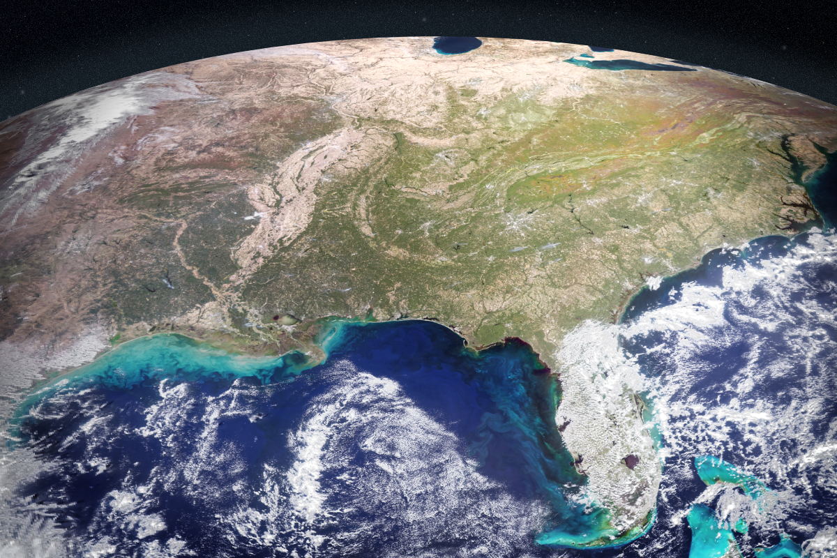
Every year, shimmering green swirls of microscopic algae—phytoplankton—paint the world’s oceans. While most are harmless, certain species can explode into harmful algal blooms (HABs), threatening human health, marine life, and coastal economies. In the Gulf of America, Karenia brevis produces potent toxins that kill fish, foul beaches, and even become airborne, causing respiratory illness. On the West Coast, Pseudo-nitzschia blooms have poisoned dolphins and sea lions. These events cost the U.S. tens of millions of dollars annually. Traditional monitoring relies on boat-based water sampling and lab analysis—a slow, expensive process that often misses blooms before they spread. To accelerate detection, NASA scientists have developed an artificial intelligence tool that fuses data from multiple Earth-orbiting satellites. Published in AGU Earth and Space Science, this tool can pinpoint HABs in regions like western Florida and Southern California, serving as a force multiplier for health agencies. This tutorial walks through the concepts and steps behind building such an AI system, from satellite data to actionable insights.

Prerequisites

Before diving into the AI pipeline, you need a solid foundation in:

• Remote Sensing Basics: Understanding how hyperspectral and multispectral satellite sensors work—e.g., NASA's PACE (Plankton, Aerosol, Cloud, ocean Ecosystem) and TROPOMI (Tropospheric Monitoring Instrument).
• Python Programming: Familiarity with data science libraries like numpy, xarray, rasterio, and scikit-learn or tensorflow for machine learning.
• Oceanography Knowledge: Knowing key HAB species (K. brevis, Pseudo-nitzschia), their spectral signatures, and environmental drivers (temperature, nutrients, currents).
• Data Access: Ability to download satellite datasets from NASA's Earthdata portal or NOAA CoastWatch.

Step-by-Step Guide

Step 1: Gather Satellite Data

NASA’s PACE satellite carries the Ocean Color Instrument (OCI), a hyperspectral sensor that captures visible light in hundreds of narrow bands. This allows it to identify phytoplankton communities by pigment, size, and shape. Meanwhile, TROPOMI aboard the Sentinel-5P satellite detects the faint red fluorescence (sun-induced chlorophyll fluorescence) emitted by certain species during photosynthesis—a telltale sign of K. brevis. To replicate the study, you’d collect:

• OCI Level-2 products: Remote sensing reflectance (Rrs) and chlorophyll-a concentration.
• TROPOMI Level-2 fluorescence data.
• Auxiliary data: Sea surface temperature (SST), wind speed, and bathymetry from NOAA or other sources.

In Python, you might load a NetCDF file from PACE like this:

import xarray as xr

oci_data = xr.open_dataset('pace_oci_l2_20241021.nc')
chl = oci_data['chlorophyll_a']

Step 2: Preprocess and Fuse Datasets

Satellites have different resolutions, orbits, and revisit times. The AI tool’s first challenge is to fuse these heterogeneous data into a consistent grid. Steps include:

1. Reprojection: Align each dataset to a common spatial reference (e.g., WGS84).
2. Resampling: Interpolate fine-resolution OCI (1 km) to match coarser TROPOMI (7 km) or vice versa.
3. Temporal collocation: Match satellite overpasses within a narrow time window (e.g., ±3 hours).
4. Cloud masking: Remove pixels contaminated by clouds or land.

The fused product becomes a multi-dimensional tensor: latitude × longitude × (spectral bands + fluorescence + SST). This serves as the input to the AI model.

Step 3: Train an AI Model

The team used a machine learning approach (likely a convolutional neural network or random forest) to classify blooms. Training requires labeled examples—areas where K. brevis or Pseudo-nitzschia blooms were confirmed via water samples. NOAA and state agencies provide these through their HAB monitoring networks. The model learns patterns in the fused satellite data that correlate with bloom presence. A simplified training loop could look like:

from sklearn.ensemble import RandomForestClassifier

# X: fused satellite features, y: bloom labels (0/1)
model = RandomForestClassifier(n_estimators=100)
model.fit(X_train, y_train)

Important: The model must be validated on independent test data to avoid overfitting. The NASA study tested on blooms in Florida and California, achieving high accuracy.

Step 4: Detect and Classify Algal Blooms

Once trained, the AI tool can process new satellite scenes in near real-time. For each pixel, it outputs a probability of HAB presence. It also distinguishes between species by analyzing the spectral signature—e.g., K. brevis shows a distinct fluorescence peak near 685 nm. The tool can generate maps over large areas (e.g., entire Gulf Coast) within minutes, rather than days. This helps health agencies prioritize where to send testing boats.

Step 5: Validate with On-Site Testing

Despite its power, the AI is not a replacement for in-water measurements. It provides a “first alert” that narrows the search area. Agencies then collect samples from flagged locations, analyze them in labs for toxin concentrations, and issue public warnings. The feedback loop—comparing AI predictions with ground truth—also improves the model over time.

Common Mistakes

• Ignoring atmospheric correction: Satellite signals are distorted by aerosols and sunlight. Use validated algorithms (e.g., NASA's SeaDAS) to convert raw radiance to water-leaving reflectance.
• Overfitting to a single region: A model trained only on Florida blooms may fail in California due to different water conditions. The NASA study explicitly tested both regions to ensure generalizability.
• Neglecting temporal dynamics: Blooms can move with currents. Incorporating SST and wind data helps the AI account for advection.
• Using low-quality labels: Water sample locations must be precisely matched to satellite pixels—a mismatch of even 1 km can introduce noise.

Summary

NASA’s new AI tool revolutionizes harmful algal bloom detection by fusing data from multiple satellites—like PACE’s hyperspectral eyes and TROPOMI’s fluorescence sensitivity—into a single predictive model. This guide walked through the essential steps: gathering satellite data, preprocessing and fusing it, training a classifier with ground-truth labels, deploying it for real-time detection, and validating with on-site sampling. The result is a faster, more efficient way to protect coastal communities and ecosystems from toxic blooms. While challenges like data integration and regional variability remain, this approach offers a scalable blueprint for global HAB monitoring.